Abstract:
The grown of investments in securities has led to higher risk and return on the investments. This paper aims at identifying the risks that are involved in the securities markets and the tools to measure the risk. The various types of returns and their relationship with each other are also discussed. The paper brings out the advantages of diversification of investments and applies the CAPM theory to the construction of an efficient portfolio. This study also involves identifying the uses and application of Capital Market Line (CML) and Efficient Portfolio curves. This paper also includes the valuation of a portfolio using the Sharpe ratio.
Keywords: Security analysis, Capital Asset Pricing Model, Capital Market Line (CML), Efficient frontier, Risk and Return, Sharpe ratio.
1.0 Introduction
“Never depend on single income. Make investment to create a second source.”- Warren Buffett. The growth of inflation and the reduction in the returns on the traditional investments has led to an increase in the investment in other forms of investments ranging from Real Estate, EFTs, Securities, And Precious metals etc. As a result if this the increase in the risk involved in investment has also significantly grown up as the returns from these investments is dependent on various factors. The returns on the modern avenues of investments like Mutual funds, ETF, Securities are not fixed like in case of Bank and post office deposits or Bonds or any debit instrument whose return is already fixed at the time of purchase of that instrument. With the inclusion of FDI and FII in the Indian Stock market the value of stocks have increased due to large demand by FDI and FII. There is a strong positive correlation between FDI & Sensex and FDI & nifty and moderate positive correlation between FII & Sensex and FII. The major drawback of investing in securities is the risk involved as the returns are not fixed. In this study the researcher has described the classification of risks and the different type of returns often discussed in securities analysis.
This paper also brings out the application of the Capital Asset Pricing Model (CAPM) in construction of an efficient portfolio with the help of SML, CML and Efficient Frontier.
CAPM was first developed by William F Sharpe, Jan Mossing and John Linter based on the modern portfolio theory given by Harry Markowitz in 1952. This paper is limited to investigation of the simple CAPM involving single period, risks and beta only. The other limitation of this study is it does not provide an insight on the business risks worldwide. It should also be noted that all the securities studied are from a single market, India and are traded over a single stock exchange (BSE). Sensex is takes as the market indicator as it shows as the movement of most of the stocks traded in the BSE. Also as this study is based on the CAPM which was developed in the late 1960s with assumptions specific to that period but the current market is different from the history the assumptions will be later discussed in this paper.
2.0 Review of literature:
Gupta (2011) conducted a comparative study of various Asian stock markets with the Indian Stock market. The Study was to identify the correlation of the returns of Indian stock market with respect to other selected stock exchanges in Asia. The study included BSE (India), KS11 (Korea), Hang Sang (Hong Kong), KLSE (Malaysia), JKS (Indonesia). The Study identified that the weekly return of Indian market and the Indonesian market was the highest at 23% and the Indian Stock market had the highest volatility indicating higher level of risk. This study was conducted in during the period between 2005 and 2009.
Do, Toan Trung (2014) in this study states that the investors prefer investment than savings to create another source of income in addition to the income they earn by working. The study states that the investor should be aware of their risk tolerance limits and the characteristics of the assets in which they invest.
Dinesh Dayani (2017) this article lists down the top ten biggest stock exchanges in the world as of November 2017. Bombay Stock Exchange (BSE), India was ranked the 10th biggest stock exchange in the world with a market capitalization of Rs1,43,82,306 Crores (US$2.22 trillion). The article also states that BSE500 has grown from 11,072.57 points to 14,494.19 points and this indicates a rough growth of 30.9% in the year 2017.
Rakesh Kumar and Raj S Dhankar (2008) Study the relationship between risk and return and also examine diversification effect on portfolio risk, which included market and non-market risk. The study was carried out daily, weekly and monthly on the basis of adjusted opening and closing prices of BSE 100 composite portfolios during the period June1996 to May 2005. The study states that Portfolio risk and return display a high degree of positive correlation in terms of Monthly returns. It is also identified that non-market risk in the portfolio tends to decline with the diversification in the portfolio.
3.0 Objectives of the study:
- To identify the risks and return in security investment
- To understand the various tools of measuring risk
- To understand Capital Asset Pricing Model and related concepts
- Valuation of portfolio using Sharpe Ratio
- Application of CAPM in portfolio construction
4.0 Research Methodology:
This paper is constructed based with the aim of constructing the optimal portfolio according to the risk level of the investors through the application of CAPM theory. This study is carried out on deductive and inductive methods. Deductive method was used to portray the different types of risks and returns in investments and on understand the advantages of portfolio diversification and CAPM theory and related concepts. Inductive method of study was used with the formulation on new hypothesis to study the effectiveness of the portfolio diversification in real life scenario and to test the effect of the constructing a portfolio based on CAPM and related tools.
The descriptive statistics was carried out by feeding the relevant data about the stock in Excel for the calculation of correlation among the securities. Other measures of risk were calculated by applying the related formulas. The efficient frontier, CML and SML were constructed using excel by adding relevant data about the securities.
5.0 RISK AND RETURN
In this chapter the researcher deals with the two major classification of Risk in securities market and elongates on the return concept which will be used in the CAPM model.
Every investor should be aware of the risk that is involved in the investments before investing. This is the fundamentals of the CAPM model as this model deals with risk free return, beta of a security and market return these concepts will be discussed in detail in the coming chapters.
5.1 Risk
There are different types of risk like business, finance, international risk etc. However with respect to the security investment the risks are classified into two risks a. System or market risk b. Unsystematic or unique risk.
5.1.1 System or Market risk:
This risk is common to the whole market and it impacts the flow and return of the market as a whole. Interest rate, Tax structure, Monetary and Fiscal policy and political stability can be quoted as examples for System or market risk.
System risk is also called as “non-diversifiable risk” or “volatility” as this category of risk is common to a major number of securities traded in a single market. To counter these risks the investor could hold a significant investments in fixed return securities which will respond differently to a major systematic change. For example: An increase in interest rates will increase the returns on the new bonds but will lead to reduction in the price of stock as the borrowing cost increases and also the return demanded of equity will increase as the risk free rate of return (discussed in later chapter) will be high. This type of risk cannot be completely eliminated through diversification alone.
The BSE Sensex fell 24.6% towards the close of 2011 an article by B. S Srinivasalu Reddy in India today mentions that this fall is primarily due to high inflation, increase in interest rates, and fall in domestic growth, depreciation local currency and other global instability in the past 12 months. This incident shows that the market risk is applicable to majority of the securities in the market.
5.1.2 Unsystematic or specific risk:
Unsystematic or specific risk is the risk associated with a particular security or investment. These risks are micro economic in nature and are related to a single asset. This risk arises due to the operational or financial risk involved in a specific company. Risks like labor strike, poor management decisions, and increase in the cost of inputs can be classified under specific risk. Apart from operational risk it also systematic risk includes financial risk like improper capital structure and poor financing decisions.
This risk is also called as diversifiable risk as this risk can be reduced by investing in different securities or multiple industries and companies. Specific risk can be reduced by constructing a portfolio where the investments are uncorrelated in terms of returns. The table given below shows the advantage of diversification for an investor.
| Number of securities | Reduction in specific risks (%) |
| 1 | 0 |
| 2 | 46 |
| 4 | 72 |
| 8 | 81 |
| 16 | 93 |
| 32 | 96 |
| 64 | 98 |
| 500 | 99 |
*Table 1-Source: Pike, R., & Neale, B. (2009). Corporate Finance and Investment: Decisions and Strategies (6th Ed.). Pearson. 231
The incident of crash of Satyam stock values after the founder and chairman of the company Ramalinga Raju confessed on 9th January 2009 that the company’s accounts were tampered and brought to light the Rs 7,136-Crore fraud carried out by him and closed circle of relatives and employees. The stock of Satyam computes fell to Rs 11:50 on Friday, the stock of the said company was traded for a high of Rs 544:00 last year (2008).
Figure 1: Stock Chart of Mahindra Satyam: (BSE: 500376 |NSE: SATYAMCOMP)
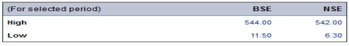
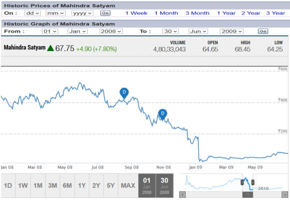
Source: Money Control 2018
5.2 Return
Return can be described as the reward for the risk the investors takes by investing in a security. With greater degree of risk the investors demand greater returns from an investment. The risk-return trade off states that the potential return rises with an increase in risk. It can observed that the major composition of the risk involved in investing in a security is the result of the volatility of the market or the systematic risk as the specific risk or unsystematic can be reduced to a large extent by diversifying the investment into different portfolios.
In this study the researcher has studied a. Risk free rate of return b. Market return and premium c. Expected return d. Actual return e. Required return
5.2.1 Risk free rate of return:
Theoretically risk free return can be defined as the return investors earn with zero risk. But practically in the globalized word of today no investment can be classified as risk free investment as even the safest of investment carry a small amount of risk and the return on these safest investments are also significantly low. Generally the securities backed by the Government are classified as risk free security and the return fixed on these securities are considered risk free rate of return. As specified that all investment involve a small amount of risk, investment in Government securities is backed by the Government so the risk of the investment depends on the credibility of the Government backing the securities.
In the year 2003 in Uruguay the Government extended the average maturity on bonds with no reduction of principle as a debit exchange as the Uruguay debt escalated to 100% of GDP. Moddy’s classified this offer as a distressed exchange/default.
For this study the interest rate on 364-Day Treasury bill (Primary) Yield of the India Government at the rate of 7.68% is considered to be risk free investment therefore the risk free rate for this study is 7.68% per annum.
5.2.2.1 Expected return:
The return an investor expects or anticipates from a portfolio on the basis the past information available about a stock. It can be calculated using computers or processed based on the information the investor receives. Expected return on a portfolio is calculated using the formula
Re = R1P1 + R2P2 + R3P3………RnPn
Re -Expected return
Rn -Return on investment “n”
Pn – Probability of the return on investment “n”
Expected return acts like a projection or an estimate of the portfolio return in the future and hence the chance of difference between the actual return and expected return can be high, it is not advisable for an investor to make a decision based on the expected return of an asset as in calculation if expected return does not incorporate the deviation of the returns over the period of time, which is a major risk component.
5.2.2.1 Expected return on a portfolio:
The return an investor expects from a portfolio consisting of more than one asset can be calculated as the weighted average of the anticipated future profits of the each asset in the portfolio. Formula for computation of expected return on a portfolio is as below.
Ep = w1R1 + w2R2 + …+ wnRn
Ep = Expected return on a portfolio
w1 = Weight or portion of asset one
R1 = Expected return on asset 1
Expected return on a portfolio does not guarantee the rate of return. It can be used as a factor in analyzing the Coefficient Variation (CV) of the portfolio.
5.2.3 Actual return:
It is the measure of the actual return the portfolio has earned over a period of time. Actual return is calculated using the formula
Ra =[(P1-P0) + D]/P0
Ra = Actual return
P1 = Value of investment at the end of the period
P0 = Value of investment at the beginning of the period
D = Dividend earned during the period (if any)
Actual return is calculated toward the end of the period as is used to identify the deviation of the return from the portfolio compared to other returns; this helps the investor to analyze the performance of the portfolio for the specified period.
5.2.4 Required return:
Required rate of return is the minimum return an investment is required to earn for an investor to invest. It can also be said that required return is the minimum return the investor demands to invest in a particular investment. CAPM can be applied to identify the required return of an investment. Required return is calculated using various factors including β (Beta) of a security, rate of inflation, risk free return and market return. This is further explained along with CAPM model in chapter 3.
6.0 MEASURES OF RISK:
Standard deviation is the tool that of often used by investors to analyze the involved in investing in an asset. Standard deviation is also referred as the volatility of the return on the asset. If an asset has high standard deviation then it is referred as a highly volatile stock i.e. the variation between the average return and actual return over the past years has been high. These assets are classified as high risk assets as it is difficult to project the future return of the asset due to its high volatile nature.
6.1 Variance and Standard deviation (Ϭ) of a portfolio:
Standard deviation is the measure of dispersion of a data from its mean. Calculation of the Standard deviation of the return of any asset will help in identifying the volatility or the risk involved in the investment. The formula to calculate a standard deviation of a single random variable can be applied to calculate the standard deviation of a single asset portfolio.
Ϭ = [(Ri – Re)2 Pi]0.5
Ϭ = Standard deviation of the asset
Ri = Actual rate of return
Re = Expected rate of return
Pi = Probability of actual return
Example:
Asset XYZ has an expected return of 10% and the actual returns for the past the years were 8%, 12% and 15% with a probability of 0.4, 0.3 and 0.3 respectively. The Standard deviation of the asset can be calculated as follows
Ϭ = [(0.08-0.1)2(0.4) + (0.12-0.1)2(0.3) + (0.15-0.1)2(0.3)]0.5 = = 3.21%
The above illustration explains that the investor can expect a deviation of +3.21% between the actual deviation and expected deviation.
Using the standard deviation the investor will be able to ascertain the volatility or the level of risk in an investment. Risk averse investors will prefer investing in low volatile securities or securities with less standard deviation. Hence, the standard deviation is also helpful in comparison of two or more assets based on the volatility.
6.2 Coefficient of variation (CV):
Another popular tool to measure the risk of an asset is Coefficient of variation. CV gives the ratio of the risk (Ϭ) as a part of expected return (Re). CV is highly helpful in comparison of two or more asset and is relatively easy provided the investor is aware of the Re and the Ϭ of the asset. CV of an asset is calculated using the formula
CV = Ϭ/Re
CV= Coefficient of variation
Ϭ = Standard deviation of the asset
Re = Expected rate of return
If two assets A and B yield the same rate of return and asset A has a higher CV than asset B it indicates that the investor is taking more risk by investing in asset A compared to asset B as asset B gives the same return for a lesser risk.
6.3 Standard deviation of portfolio with two or more assets:
The return on a portfolio can be calculated as the sum of the product of the weights or portion of each asset in the portfolio to the respective return of each asset. This same concept cannot be applied while calculating the portfolio standard deviation. The calculation of portfolio standard deviation includes the covariance abound the different assets in the portfolio. If the assets are perfectly correlated i.e. correlation between the assets is 1 then a simple weighted average of the variance will work. But in most cases it very rare to have assets with a correlation of 1. Hence, we take into account the covariance of the assets into the equation.
6.3.1 Covariance measures how the assets move together in the market. The assets could have positive covariance (move in the same direction) or negative covariance (move in the opposite direction). By applying the covariance of the assets the investor will be able to compute the Correlation Coefficient among the assets. Covariance (Cov) of the assets can be computed using the below formula.
Covij= Ʃ [(Ri – Average return on (i)) * (Rj – Average return on (j))] / n-1
Covij = Covariance of the assets i and j
Ri = Return on asset i
Rj = Return on asset j
n = Total number of samples
6.3.2 Correlation Coefficient:
The calculation of covariance between two stocks shows the direction in which each stock move respect to the other stock. The major limitation about the covariance is that, it helps the investor to identify the direction of asset movement with respect to the other asset but do not specify the strength of the relationship. In order to reduce the specific risk or unique risk or for an effective application of diversification of the portfolio the investor should holds assets which are negatively correlated i.e. move in opposite direction. Though, covariance helps in identifying the direction of change Correlation Coefficient assists in analyzing the strength of the relationship. Therefore, Correlation should be used along with covariance to determine the strength of the relationship. Correlation Coefficient is calculated as follows.
Correlation (i, j) = ρij = Covij / Ϭi * Ϭj Covij = Covariance of the assets i and j
Ϭi = Standard deviation of asset i
Ϭj = Standard deviation of asset j
6.3.2 Standard deviation of a portfolio:
The standard deviation of a portfolio with more than one asset depends on the standard deviation of each asset, the proportion of each asset in the portfolio, the covariance of the assets. Standard deviation of the portfolio is given calculated by applying the below formula.
Ϭp = (Wi2Ϭi2 + Wj2Ϭj2 + 2*Wi*Wj*Covij)0.5
Ϭp = Standard deviation of the portfolio
Wi2 = Proportion of asset i (squared)
Ϭi2 = Standard deviation of the asset i (squared)
Wj2 = Proportion of asset j (squared)
Ϭj2 = Standard deviation of the asset j (squared)
Wi = Proportion of asset i
Wj = Proportion of asset j
Covij = Covariance of assets i and j
Illustration:
The researcher has chosen two securities a. Maruti Suzuki India (MARUTI) and b. Tata Consultancy Services (TCS). Information about the stock is as below.
| Table 2 – Portfolio of two securities and their measures of risk | ||
| Secuities | MARUTI (i) | TCS (j) |
| Standard deviation | 1.15% | 0.839% |
| Weight of the security | 0.5 | 0.5 |
| Covariance | 0.0002 | |
| Correlation Coefficient | 0.0367 |
*Data for covariance collected from “Top stock research”. Calculations in appendix
Standard deviation of the portfolio:
Ϭp = (Wi2Ϭi2 + Wj2Ϭj2 + 2*Wi*Wj*Covij)0.5
= [(0.5)2(0.0115)2 + (0.5)2(0.008369)2 + 2*0.5*0.5*0.0002)0.5 = 0.012 or 1.2%
Expected return on the portfolio, Re = 0.19% + 2.27% = 2.46%
CV = Ϭ/Re = 1.2/2.46 = 0.4878
From the above calculations it can be interpreted that the risk involved in the portfolio is 1.2% and the expected return is 2.46%. The Correlation Coefficient is 0.0367 and the Covariance is 0.0002. The covariance shows that the assets move in the same direction but on examining the Correlation Coefficient it can be identified that the relationship between these two assets is very weak hence diversification of the investment in these two assets will lead to reduction and risk and provides the investor with the benefits of diversification.
7.0 CAPITAL ASSET PRICING MODEL (CAPM)
The CAPM guides the investor in constructing a portfolio. By applying CAPM and the related concepts the investor will be able to know the maximum return at a specified level of risk or the minimum risk one should take to earn a said rate of return. CAPM was developed after 12 years from the development of the Portfolio diversification model developed by Harry Markowitz in 1952. This model helps the investor to decide on the how to apply the concept of diversification i.e to select the best mix of different assets in a portfolio. In order to understand the model the investor must be aware of the underlying concepts in CAPM. In this paper the researcher discusses on a. Marker return and Market risk premium (Rm) b. Beta of the stock (β) c. Expected return on an asset (Re) d. Efficient Frontier e. Capital Market Line (CML)
7.1 Market Return (Rm) and Market Premium:
Market portfolio consists of the entire stock that is available to the investor, it is the aggregate of all the securities or investment avenues available in the entire economy. The return expected by an investor from the market portfolio is Market return. As the specific risk can be eliminated to a large extent by implementing diversification technique and selecting the right combination of assets the return of an asset is the greatly influenced by the Market risk or Systematic risk. Market return is generally calculated on the index of stock markets as they show a broader picture of the market trend. S&P 500 is a popular index that is used by analysts to study the past returns in a market and project the future. The market return will differ from one investor to the other based on the index they use for analysis and the investors expectation from the market. The market return for this study is calculated on the basis of BSE Sensex which is composed of the 30 most actively traded stocks in BSE. Sensex is composed of 30 of the largest and most actively-traded stocks on the BSE, providing an accurate gauge of India’s economy. The return on the market was considered to be 15.2% annually.
7.1.1 Market premium is the excess of return the market portfolio delivers over the risk free return. In other words it can be defined as the excess of return investors receives over the risk free rate of return by investing the money in the market over risk free securities. Market premium or risk premium is an important factor to be employed in application of CAPM model. Formula for calculation of Market premium (MP).
MP = Rm-Rf
MP = Market premium
Rm = Market return
Rf = Risk free return
7.2 Beta of the stock (β):
It measures the relation between of a particular asset and the market portfolio. It is a measure of volatility, or systematic risk of an asset. The beta of a stock measures the extent to which returns on a stack and the market move together. The Beta of a stock can be interpreted as follows. If the Beta of a stock is 1, it shows that the asset moves perfectly along the market with no deviation. A beta value of less than one can be interpreted as, the volatility of the stock is less than the volatility in the market and a beta value of more than one shows that the stock is more volatile than the market.
Example: If a company is said to have a beta of 1.5 the investors in this company can expect a return of 150% of market return i.e. if the market return is 12% the investor can expect 18% (12* 150/100) from this company. It also indicates that if the market is falling the investor in this company will lose 150% of the market i.e. If the market has a return of -6% the investor in this company will expect -9% [(-6)*150/100]. If a company is said to have a beta of 0.65 the investor in this company can expect a 65% of the market return. A higher beta shows that the stock will bring higher return than the market but it also has a higher magnitude of loss if the market falls.
Beta of a security can be calculated using the below formula
β = Cov (i,m) / (Ϭm)2
β = Beta of the security
Cov(i,m) = Covariance of the security and the market
(Ϭm)2 = Variance of market
7.3 Expected return on an asset (Re):
CAPM model guides the investor to decide on the optimal portfolio which is expected to earn a specific rate of return with minimum risk. The expected return on an asset is the return the investor is expected to earn from the asset in the future. The formula to calculate the expected rate of return on an asset is as follows.
Re = Rf + β(Rm- Rf)
Re = Expected return on an asset
Rf = Risk free rate of return
β = Beta of the asset
Rm= Expected return on the market
From the formula it can be identified that the expected rate of return on an asset is the sum of the risk free rate (Rf) and the product of the asset’s volatility compared with the market (β) and the addition risk the investor accepts by investing in the market over the risk free assets i.e. Market premium (Rm- Rf).
7.4 Efficient Frontier:
In the process of construction of a portfolio using multiple assets the investor will have plenty of was to combine the different assets or to allocate the capital which is a limited resource among different asset. The allocation of capital depends significantly in the risk tolerance level of the investor. A risk averse investor will prefer to have more of assets with low level of volatility. The efficient portfolio is the combination which will yield the highest return for a specified rate of risk. For every level of risk there exists an efficient portfolio which will give the highest return at that specific level of risk.
Figure 2 Optimal portfolio:
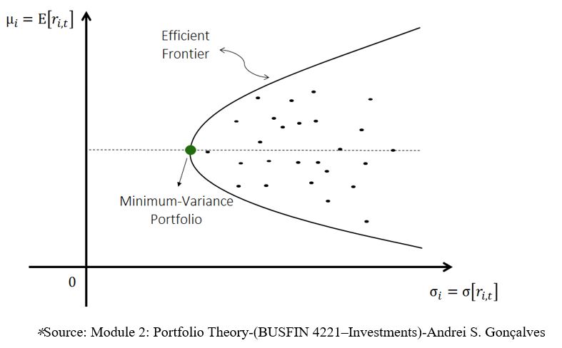
In the Figure 2, the graph shows the various combination of assets an investor can hold and the assets or portfolios are plotted by taking the risk (Ϭ) involved in the portfolio along the X-axis and the expected return (Re) on Y-axis. On the graph the point where the risk is minimum for the different combination of the asset is called the Minimum variance portfolio. It is also called as the minimum risk portfolio and also represents the best diversification possible as it reduces the risk as low as possible. As we plot all the portfolios which yield the maximum return at a specified level of risk to the right of the minimum variance portfolio we see the efficient frontier as shown in the figure. At a given level of risk the maximum return an investor can expect falls on the efficient frontier, at least when short selling is allowed. All the assets and combination of assets which fall below the efficient frontier are considered to be sub-optimal as there is an optimal combination which falls on the efficient frontier. Therefore, every portfolio that appears on the efficient frontier is called Optimal Portfolio as they show the highest expected return for a specific level of risk given by the investor.
7.5 Capital Market Line (CML)
The different combination of risky assets which gives the highest return at a specific level of risk can be identified using the efficient frontier. The efficient frontier consider only the risky assets but in real word the investor can also invest in risk free securities like Treasure Bills which are not included in construction of an efficient frontier as these assets are classified as risk free asset as they are backed by the Government. In order to include the risk free assets in construction of a portfolio the investor is guided by the Capital Allocation Line (CAL) and Capital Market Line (CML). Theoretically CALs consists of all possible combination of risky and risk free assets for different levels of expected returns of an investor. The slope of the CAL is constructed using the formula
ERp = Rf + [(ERp – Rf)/ Ϭp] *Ϭnp
ERp = Expected return on the portfolio
Rf = Risk free rate of return
Rm = Expected return on the combined risky assets
Ϭnp = Standard deviation of the new portfolio (including risk-free assets)
Ϭp = Standard deviation of the combined risky assets
7.5.1 Relationship between Capital allocation line (CAL) and Efficient frontier:
For every combination of risky assets a capital allocation line can be constructed and the slope of the line is influenced by the excess return the portfolio gives over the risk free return and the risk involved in the combinations.
Figure 2:
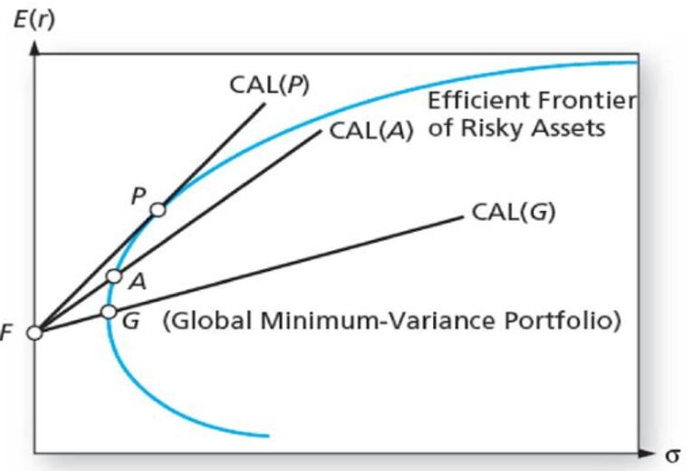
* Source: Figure 7.13 Capital allocation lines with various portfolios from the efficient set. (Investments- Bodie, Kane and Marcus
In the above figure it can be observed that there three CAL i.e CAL (G) for Portfolio G, CAL (A) for Portfolio A and CAL (P) for Portfolio P. CAL (P) is the steepest of the three lines and has the highest slop of the three which indicated that the portfolio on this line is the most optimal combination of risky and risk free asset of the whole frontier i.e. At this combination the investor is expected to earn the highest with a relatively low return. It can also be narrated that at Portfolio P the risk return trade-off is the best as CAL represents the risk return trade-off of a portfolio and every other CAL will remain below the CAL (P). CAL (P) which offers the highest risk return tradeoff is referred as the Capital Market Line (CML). Portfolio P is also called the Tangency portfolio or Mean Variance Efficient portfolio (MVE).
8.0: VALUATION OF PORTFOLIO USING SHARPE RATIO
The Sharpe Ratio was developed by Nobel laureate William F. Sharpe. Sharpe ratio give the excess return the portfolio offers over the risk free rate for every unit of risk taken by the investor. A portfolio higher with a higher Sharpe ratio indicates that the portfolio return as better return for the risk as compared with a portfolio with the lesser Sharpe ratio. The slope of the CML is the highest Sharpe ratio possible because at the combination of the portfolio which falls on the CML i.e. Tangency Portfolio offer the best risk return trade off to the investor. The Sharpe ratio is calculated using the formula
Sp = (ERp – Rf) / Ϭp
Sp = Sharpe ratio
Rf = Risk free rate of return
Rm = Expected return on the combined risky assets
Ϭp = Standard deviation of the combined risky assets
9.0 CONSTRUCTION OF COMPLETE OPTIMAL PORTFOLO
For the purpose of this study the researcher has chosen three assets which are traded in Bombay Stock Exchange (BSE). The monthly returns on these securities for the past year since Sept 2017 to Aug 2018 was used to construct the portfolio.
9.1 Steps in construction of a complete optimal portfolio:
Step 1: As a first step the researcher constructed an efficient frontier which demonstrates the risk and return for different combination of the three securities
Step 2: In this step the researcher identified the slop of the CML i.e. the combination having the highest Shape ratio
Step 3: Post the identification of the portfolio with the highest Sharpe ratio, CAL which is corresponding to that portfolio was constructed using Excel. This CAL is also the CML as this has the highest slope or Sharpe ratio compared to other combinations.
Step 4: To decide on the proportion to be invested in risky asset the below formula is applied
y = (ERp – Rf)/A*Ϭp
y= Proportion to be invested in risky assets
ERp = Expected return on the portfolio
Rf = Risk free rate of return
Ϭp = Standard deviation of the combined risky assets
A = Risk aversion of the investor. It is usually measured in a scale of 1 to 5 with 1 being highly averse to risk and 5 being less risk averse. A person who is neutral to risk will have a risk aversion value of 0
Step 5: Once the proportion of risky assets is decided the remaining amount to be invested in risk free security is identified by subtracting it from the entire fund available for investment
Step 6: This is the last step where the investor will apportion the amount kept allocated for risky assets in proportion to the optimal portfolio identified and the remaining in the risk free asset
9.2 Construction of optimal portfolio among the chosen securities:
| Table 3 – Correlation of securities | |||
| HDFC | Sun Pharma | Coal India | |
| HDFC | 1.0000 | -0.3594 | 0.1180 |
| Sun Pharma | -0.3594 | 1.0000 | 0.0416 |
| Coal India | 0.1180 | 0.0416 | 1.0000 |
* Source of data and calculation attached in appendix
| Table 4 – Covariance of securities | |||
| HDFC | Sun Pharma | Coal India | |
| HDFC | 0.0019 | -0.0013 | 0.0004 |
| Sun Pharma | -0.0013 | 0.0068 | 0.0003 |
| Coal India | 0.0004 | 0.0003 | 0.0058 |
*Source of data and calculation attached in appendix
From the above calculations it can be interpreted that the three securities will be able to provide the investor with the benefits of diversification as the correlation among these securities are considerably less ranging from -0.3594 and 0.1180.
Chart 1: Identification of Efficient frontier and CML
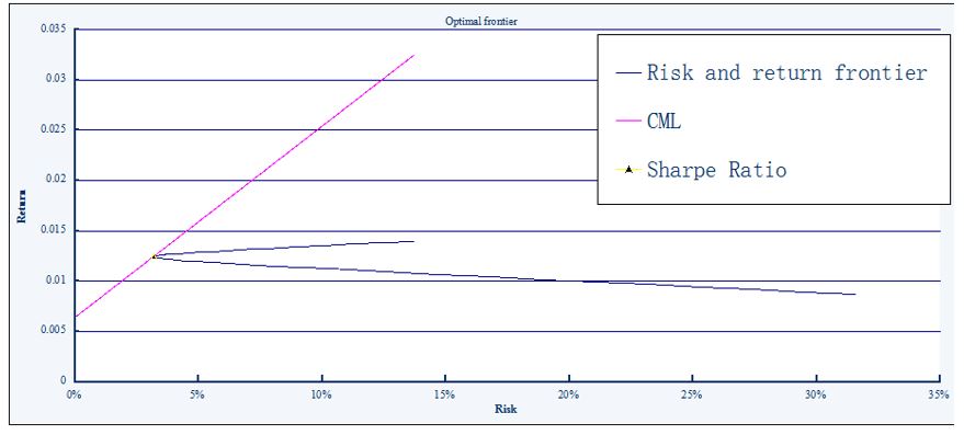
*Source: Developed by author. Data in appendix
Chart 2 Tangency portfolio:
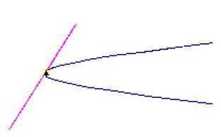
*Source: Chart 1
| Table 5: Tangential portfolio | ||||||
| HDFC | Sun Pharma | Coal India | Risk | Expected return | CML | Sharpe ratio |
| 53.82% | 33.36% | 12.82% | 3.169% | 1.244% | 1.244% | 0.19059 |
* Source Developed by author, data in appendix
From the analysis it is identified that the above portfolio has the highest Sharpe ratio of all the combination and from the chart it can also be identified that the CAL respective to this portfolio is tangential to the frontier hence it is the CML of the frontier. Therefore it can be said that the above portfolio is the optimal portfolio for the combination of these securities.
9.3 Complete optimal portfolio of the case:
If the investor has a risk aversion value of 4 the complete optimal portfolio at this point is calculated as below.
9.3.1 Calculation of proportion of amount to be invested in risky assets:
y = (ERp – Rf )/A*Ϭp
ERp = 1.244%
Rf = 0.64%
Ϭp = 3.169%
A = 4
y = 47.85%
Therefore in the complete optimal portfolio the investor holds 47.85% of funds in risk free assets and 52.15% of funds in risky assets. The portfolio constructed will appear as follows.
| Table 6: Completely optimal portfolio | ||||||
| HDFC | Sun Pharma | Coal India | Risk free | Expected return | Portfolio risk | Sharpe ratio |
| 28.07% | 17.04% | 6.69% | 47.85% | 1.29% | 1.630% | 0.39518 |
*Source: Developed by author
It can be observed that with the addition of risk free asset to the portfolio the investor is able to enjoy a better risk return tradeoff. The inclusion of risk free assets reduces the risk by a significant level and it is reflected by increase in Sharpe ratio. It can be noted that the Sharpe ratio of optimal complete portfolio is greater than the optimal portfolio with risky assets alone.
| Table 7 – Observation of Completely optimal portfolio from 01.09.2018 to 21.09.2018 | ||||
| Particulars | HDFC | Sun Pharma | Coal India | Risk free |
| Closing 21st Sept | 1,970.25 | 634.90 | 275.25 | |
| Opening 1st Sept | 2,062.25 | 652.20 | 286.10 | |
| Portion of investment | 28.07% | 17.04% | 6.69% | 48.20% |
| Investment in (Rs) | 28,070.00 | 17,040.00 | 6,690.00 | 48,200.00 |
| No. of stock | 13 | 25 | 22 | |
| Value of investment (opening) | 26,809.25 | 16,305.00 | 6,294.20 | |
| Value of investment (Closing) | 25,613.25 | 15,872.50 | 6,055.50 | |
| Loss on investment | 1,196.00 | 432.50 | 238.70 | |
| Gain on Investment | 215.94 | |||
| Net Loss on portfolio | 1,651.26 |
*Source: Developed by author. Opening and closing balances of securities collected from economictimes.indiatimes.com
| Table 8 – Observation of Portfolio without diversification from 01.09.2018 to 21.09.2018 | |||
| Particulars | HDFC | Sun Pharma | Coal India |
| Closing 21st Sept | 1,970.25 | 634.90 | 275.25 |
| Opening 1st Sept | 2,062.25 | 652.20 | 286.10 |
| Portion of investment | 100.00% | 100.00% | 100.00% |
| Investment in (Rs) | 100,000.00 | 100,000.00 | 100,000.00 |
| No. of stock | 48 | 153 | 350 |
| Value of investment (opening) | 100,000.00 | 100,000.00 | 100,000.00 |
| Value of investment (Closing) | 95,538.85 | 97,347.44 | 96,207.62 |
| Loss on investment | 4,461.15 | 2,652.56 | 3,792.38 |
* Source: Developed by author. Opening and closing balances of securities collected from economictimes.indiatimes.com
On comparing the table 7 and 8 the researcher was able to see that the loss on the completely optimal portfolio is considerably less compared to a single asset portfolio. Hence, it can concluded that the CAMP model holds good with respect to the securities included in the study traded in BSE for the period 1st Sept 2018 to 21st Sept 2018.
10.0 Assumptions and limitations of the study:
This study was conducted based on the assumptions of the CAPM model and certain assumption of CAPM that has strong limitation in this study are
- All investors are rational and expect maximum with minimum risk – Not all investors fall under this category as the market is greatly influenced by speculators
- The securities can be traded in fractions for any amount – This assumption is not always true as securities can be traded in fractions
- In reality every investment included a small amount of risk hence practically there is no risk free investment
- This study assumes that there is no tax rate or transaction cost but this assumption is far from reality as taxes are applicable on the returns from investment and different level of taxes apply depending on the nature of return. The investor has to pay brokerage and transaction fee for carrying trading in securities.
10.1 Other limitations:
- This study was limited to three securities from the same market (BSE)
- This study does not practically test the efficiency of the results with a real life market situation over a longer period of time
- The calculations in this study are based on past 12 months only hence it does not provide a long term trend of the securities
- Monthly returns on the securities was considered as the basis for calculation, monthly returns do not provide the actual trend in the value of securities
11.0 Findings of the study:
- Risks involved in investments are broadly classified into systematic risk and unsystematic or specific.
- Specific risks involved in an investment can be reduced significantly by diversifying the investments among different investment avenues
- The standard deviation of returns from an investment is primarily considered as a measure if risk of the investment
- In order to maximize the advantage of diversification the investor should hold securities that are less correlated among each other
- All portfolios that lay on the efficient frontier are superior to the portfolios that appear below the efficient frontier
- The CAL that is tangential to the efficient frontier carries the highest slope and is called as CML
- Portfolio corresponding to the CML is identified to be the best portfolio mix as at this point the Sharpe ratio is maximum
- Sharpe ratios shows the risk return tradeoff of the portfolio. Higher Sharpe ratio of a portfolio shows that the investor is able to get more return for the risk involved compared to a portfolio with low Sharpe ratio
- To construct a complete optimal portfolio which included risk free assets the investor’s risk aversion value is considered
- A complete optimal portfolio has a better Sharpe ratio as the risk is reduced due to a part of investment being made in risk free assets
12.0 Conclusion:
CAPM was an important theory developed over the portfolio diversification. Though this theory has its limitations bases on its assumption it is still a very popular tool used by investors and analysts in construction of a portfolio. From this study we can understand that the investor can maximize the return and minimize the risk by practicing the concept of diversification. From this study we see that the expected return on a portfolio depends on the risk of the portfolio and the risks aversion of the investor. This model helps the investor to construct a portfolio but does not guarantee the actual return as the return is determined by the investors psychology and the performance of the company, industry and the economy. In the present times of globalize economic it makes it even more difficult for the investors and analysts in construction and management of a portfolio due to the wide range of investment avenues. Each investment avenue needs to be thoroughly studied before the investment is made. Globalization has also increased the complexity of measuring the risk in each market and as every economy is connected at the global level the risk of one market is reflected across the globe.
This model can be used as a guide in construction of the optimal portfolio but it should be supported with proper fundamental and technical analysis of the securities that are included in the portfolio. A portfolio constructed using this model does not guarantee the return but with continuous analysis, and valuation of the portfolio the investor will be able to maximize the return and minimize the risk in the investment.
Appendix
| Table 9: Calculation of Co variance and Correlation Coefficient | |||||||
| Monthly return (Actual) | Expected return | ||||||
| Month | Maruti (Rs) | TCS (Rs) | Maruti (%) | TCS (%) | Probability | Maruti (%) | TCS (%) |
| 30-Sep-18 | -697.25 | -7.65 | -7.67% | -0.37% | 0.0909 | -0.70% | -0.03% |
| 31-Aug-18 | -424.15 | 138.2 | -4.46% | 7.12% | 0.0909 | -0.40% | 0.65% |
| 31-Jul-18 | 694.95 | 92.45 | 7.87% | 5.00% | 0.0909 | 0.72% | 0.45% |
| 30-Jun-18 | 288.4 | 106.7 | 3.38% | 6.13% | 0.0909 | 0.31% | 0.56% |
| 31-May-18 | -277.75 | -25 | -3.15% | -1.42% | 0.0909 | -0.29% | -0.13% |
| 30-Apr-18 | -46.15 | 341.48 | -0.52% | 23.97% | 0.0909 | -0.05% | 2.18% |
| 31-Mar-18 | 10.15 | -92.96 | 0.12% | -6.13% | 0.0909 | 0.01% | -0.56% |
| 28-Feb-18 | -658.75 | -38.65 | -6.93% | -2.48% | 0.0909 | -0.63% | -0.23% |
| 31-Jan-18 | -219.85 | 205.58 | -2.26% | 15.22% | 0.0909 | -0.21% | 1.38% |
| 31-Dec-17 | 1,130.45 | 32.1 | 13.15% | 2.44% | 0.0909 | 1.19% | 0.22% |
| 30-Nov-17 | 387.85 | 6.5 | 4.72% | 0.50% | 0.0909 | 0.43% | 0.04% |
| Standard deviation | 0.061 | 0.082 | Total | 0.39% | 4.54% | ||
| Covariance | 0.0002 | Weight | 0.5 | 0.5 | |||
| Correlation Coefficient | 0.0367 | Expected return | 0.19% | 2.27% |
* Source: Developed by author
*Data collected from “Top Stock Research” on monthly basis
*Probability in the data above is assumed by the author as (1/11 = 0.0909)
| Table 10: Construction of optimal portfolio | ||||||
| Particulars | HDFC | Sun Pharma | Coal India | |||
| Month | Closing (Rs) | % of MR | Closing (Rs) | % of MR | Closing (Rs) | % of MR |
| 17-Aug | 1,775.00 | – | 480.35 | – | 238.00 | – |
| 17-Sep | 1,803.05 | 1.580% | 503.20 | 4.757% | 270.60 | 13.697% |
| 17-Oct | 1,808.80 | 0.319% | 553.40 | 9.976% | 286.35 | 5.820% |
| 17-Nov | 1,852.05 | 2.391% | 539.95 | -2.430% | 276.20 | -3.545% |
| 17-Dec | 1,873.55 | 1.161% | 570.80 | 5.713% | 263.00 | -4.779% |
| 18-Jan | 2,006.35 | 7.088% | 579.35 | 1.498% | 298.60 | 13.536% |
| 18-Feb | 1,883.80 | -6.108% | 535.35 | -7.595% | 309.55 | 3.667% |
| 18-Mar | 1,891.45 | 0.406% | 495.40 | -7.462% | 283.50 | -8.415% |
| 18-Apr | 1,944.60 | 2.810% | 528.15 | 6.611% | 283.85 | 0.123% |
| 18-May | 2,136.15 | 9.850% | 480.15 | -9.088% | 294.50 | 3.752% |
| 18-Jun | 2,108.05 | -1.315% | 560.55 | 16.745% | 264.40 | -10.221% |
| 18-Jul | 2,181.05 | 3.463% | 566.65 | 1.088% | 261.70 | -1.021% |
| 18-Aug | 2,062.25 | -5.447% | 652.20 | 15.098% | 286.10 | 9.324% |
| β | 0.93 | 0.63 | 0.85 | |||
| Expected Return | 1.223% | 1.035% | 1.173% | |||
| Risk | 4.319% | 8.219% | 7.587% |
* Source: Developed by author
* Data source BSE India – http://www.bseindia.com
| Table 11: Risk, Return and Sharpe ratio of various combination of the three assets: | ||||||
| HDFC | Sun Pharma | Coal India | Risk | Expected return | CML | Sharpe ratio |
| 0.00% | 0.00% | 0.00% | 0.000% | 0.64% | 0.64% | 0.00000 |
| 100.59% | 132.82% | -133.41% | 13.669% | 1.399% | 3.245% | 0.05550 |
| 96.14% | 123.35% | -119.48% | 12.467% | 1.384% | 3.016% | 0.05967 |
| 91.68% | 113.88% | -105.56% | 11.272% | 1.369% | 2.788% | 0.06469 |
| 87.23% | 104.40% | -91.63% | 10.088% | 1.354% | 2.563% | 0.07082 |
| 82.77% | 94.93% | -77.70% | 8.920% | 1.340% | 2.340% | 0.07844 |
| 78.32% | 85.46% | -63.78% | 7.773% | 1.325% | 2.121% | 0.08812 |
| 76.09% | 80.72% | -56.81% | 7.211% | 1.318% | 2.014% | 0.09396 |
| 73.86% | 75.99% | -49.85% | 6.660% | 1.310% | 1.909% | 0.10064 |
| 71.64% | 71.25% | -42.88% | 6.121% | 1.303% | 1.807% | 0.10829 |
| 69.41% | 66.51% | -35.92% | 5.599% | 1.296% | 1.707% | 0.11707 |
| 67.18% | 61.78% | -28.96% | 5.099% | 1.288% | 1.612% | 0.12710 |
| 64.95% | 57.04% | -21.99% | 4.629% | 1.281% | 1.522% | 0.13844 |
| 62.73% | 52.30% | -15.03% | 4.197% | 1.273% | 1.440% | 0.15093 |
| 60.50% | 47.57% | -8.07% | 3.817% | 1.266% | 1.367% | 0.16402 |
| 58.27% | 42.83% | -1.10% | 3.506% | 1.259% | 1.308% | 0.17647 |
| 56.04% | 38.10% | 5.86% | 3.284% | 1.251% | 1.266% | 0.18617 |
| 53.82% | 33.36% | 12.82% | 3.169% | 1.244% | 1.244% | 0.19059 |
| 51.59% | 28.62% | 19.79% | 3.173% | 1.237% | 1.245% | 0.18801 |
| 49.60% | 24.33% | 26.07% | 3.279% | 1.230% | 1.265% | 0.17993 |
| 45.38% | 15.51% | 39.11% | 3.763% | 1.216% | 1.357% | 0.15310 |
| 43.23% | 10.90% | 45.87% | 4.122% | 1.209% | 1.426% | 0.13804 |
| 41.58% | 7.17% | 51.25% | 4.446% | 1.203% | 1.487% | 0.12669 |
| 40.11% | 3.97% | 55.92% | 4.749% | 1.198% | 1.545% | 0.11756 |
| 38.70% | 1.12% | 60.17% | 5.037% | 1.194% | 1.600% | 0.10995 |
| 37.53% | -1.63% | 64.10% | 5.316% | 1.190% | 1.653% | 0.10339 |
| 36.28% | -4.11% | 67.83% | 5.585% | 1.186% | 1.704% | 0.09771 |
| 26.16% | -25.37% | 99.21% | 8.042% | 1.153% | 2.173% | 0.06374 |
| 17.43% | -43.86% | 126.43% | 10.312% | 1.124% | 2.605% | 0.04692 |
| 9.25% | -61.38% | 152.13% | 12.511% | 1.097% | 3.024% | 0.03650 |
| 1.28% | -78.36% | 177.08% | 14.670% | 1.070% | 3.436% | 0.02932 |
| -6.46% | -95.12% | 201.58% | 16.810% | 1.044% | 3.844% | 0.02405 |
| -14.22% | -111.60% | 225.82% | 18.933% | 1.019% | 4.248% | 0.02000 |
| -21.74% | -128.10% | 249.85% | 21.051% | 0.993% | 4.652% | 0.01677 |
| -29.41% | -144.36% | 273.77% | 23.157% | 0.968% | 5.053% | 0.01415 |
| -36.96% | -160.61% | 297.57% | 25.260% | 0.943% | 5.454% | 0.01198 |
| -44.60% | -176.72% | 321.32% | 27.356% | 0.917% | 5.854% | 0.01014 |
| -52.13% | -192.86% | 344.99% | 29.451% | 0.892% | 6.253% | 0.00857 |
| -59.77% | -208.87% | 368.64% | 31.540% | 0.867% | 6.651% | 0.00721 |
* Source: Developed by author based on template available at
people.maths.ox.ac.uk/~howison/o10/excel/portfolio.xls (Retrived on 23 July 2019)
| Table 12: Constants used in construction of CML | |
| Market price of risk (Slope) | 0.19059 |
| Risk free rate | 0.64% |
*Source: Developed by author for the purpose of research
References
- Impact of Flow of FDI & FII on Indian Stock Market Dr. Syed Tabassum Sultana, Prof. S Pardhasaradhi
- Nupur Gupta, Comparative Study of Distribution of Indian Stock Market with Other Asian Markets. International Journal of Enterprise Computing and Business Systems, ISSN (Online): 2230-8849, Vol. 1 Issue 2 July 2011.
- CAPITAL ASSET PRICING MODEL IN BUILDING INVESTMENT PORTFOLIO
Case: A comparison between two portfolios combine stocks from same and different industries. LAHTI UNIVERSITY OF APPLIED SCIENCES, Degree program in International Business, Thesis, Autumn 2014
- 10 Biggest Stock Exchanges In The World: Here’s How Much They’ve Gained In 2017
- Rakesh Kumar and Raj s Dhankar (2008) Portfolio Performance in relation to Risk and Return and effect of diversification: A test of market efficiency, Applied Finance, IUP Publications New Delhi
- TIMELINES Satyam Scandal: Who, what and when, April 09, 2015 13:35 IST, The Hindu
https://www.thehindu.com/specials/timelines/satyam-scandal-who-what-and-when/article10818226.ece
- Indian IT scandal boss arrested – 9 January 2009 – Business – BBC NEWS
http://news.bbc.co.uk/1/hi/business/7821087.stm
- Investopedia 2018-Risk-Return Tradeoff
https://www.investopedia.com/terms/r/riskreturntradeoff.asp
- Sovereign Default and Recovery Rates, 1983-2007, Moddy’s Global Credit research, March 2008
- Cash Reserve Ratio and Interest Rates, Reserve bank of India, 14 Sept 2018
- Investopedia (2018), Expected Return, Variance And Standard Deviation Of A Portfolio
https://www.investopedia.com/walkthrough/corporate-finance/4/return-risk/expected- return.aspx
- Finance Formulas, Total Stock Return
http://financeformulas.net/Total-Stock-Return.html
- 4.2 Mean or Expected Value and Standard Deviation, Texas gateway
Resource ID:uhZIavb_@7
https://www.texasgateway.org/resource/42-mean-or-expected-value-and-standard-deviation
- Calculating covariance for stocks By Peter Cherewyk | Updated April 24, 2018 | Investopedia 2018
https://www.investopedia.com/articles/financial-theory/11/calculating-covariance.asp
- Investopedia (2018)-Correlation Coefficient
https://www.investopedia.com/terms/c/correlationcoefficient.asp
FinancialManagementProStandard Deviation of Portfolio-Yuriy Smirnov Ph.D. http://financialmanagementpro.com/standard-deviation-of-portfolio/
- Beta/Volatility of Maruti Suzuki India (MARUTI) on Daily/ Weekly/ Monthly Period
- Beta/Volatility of Tata Consultancy Services (TCS) on Daily/ Weekly/ Monthly Period
- Investopedia (2018), Sensex
https://www.investopedia.com/terms/s/sensex.asp#ixzz5RN5ZJNU2
- India Stock Market Valuations and Expected Future Returns – Updated at Sat, 22 Sep 2018
https://www.gurufocus.com/global-market-valuation.php?country=IND
- CFI-What is the Market Risk Premium?
https://corporatefinanceinstitute.com/resources/knowledge/finance/market-risk-premium/
- Investopedia 2018 – Beta
https://www.investopedia.com/terms/b/beta.asp
- Investments- Bodie, Kane, Marcus and Mohanty, 6th edition, Pg 291
- What Is the Formula for Calculating Beta? | Investopedia | By Steven Nickolas | Updated April 19, 2018
https://www.investopedia.com/ask/answers/070615/what-formula-calculating-beta.asp#ixzz5RZOkwNY5
- Investopedia 2018 – Capital Asset Pricing Model – CAPM
https://www.investopedia.com/terms/c/capm.asp
- Module 2: Portfolio Theory-(BUSFIN 4221 – Investments)-Andrei S. Gonçalves
- Capital Market Line – Obaidullah Jan, ACA, CFA, last modified on Apr 5, 2018
https://xplaind.com/282223/capital-market-line
- Sharpe Ratio – Investopedia (2018)
https://www.investopedia.com/terms/s/sharperatio.asp
- Investments-6thedition – Bodie, Kane, Marcus, Mohanty – (Pg. 218)
